
Maarten van Kampen previously caused a retraction of a Nature Communications paper (which still hasn’t happened), and now he writes about a retraction in Nature which already happened, to give you the scientific background of the fraud which the expert editors and peer reviewers at this most exclusive elite journal didn’t notice at that time because this is how broken scholarly publishing is.

Anatomy of a Retraction
From “analysis and conclusion of our paper remain valid” via drafted correction to “the authors retract this publication”. A guest post by Maarten van Kampen.
On 26 September 2022, this 2 year-old Nature paper has just been retracted, despite protests of all of its US-based authors at University of Rochester and University of Nevada Las Vegas. It announced the discovery of the holy grail of engineering: a room-temperature superconducting material, and was therefore at that time celebrated as a tremendous scientific breakthrough.
Elliot Snider , Nathan Dasenbrock-Gammon , Raymond McBride , Mathew Debessai , Hiranya Vindana , Kevin Vencatasamy , Keith V. Lawler , Ashkan Salamat, Ranga P. Dias Room-temperature superconductivity in a carbonaceous sulfur hydride Nature (2020) doi: 10.1038/s41586-020-2801-z
The last author Ranga Dias was even appointed as one of Time‘s 100 Next of 2021, meaning one of humanity’s greatest “emerging leaders” in science. In his home country Sri Lanka, media started to talk about the Nobel Prize for the nation’s greatest scientist:
“Professor Dias is not a new face in the scientific community. In 2016 and 2017 he played a major role in discovering Atomic Metallic Hydrogen H2 (solid), the rarest metal on earth and also the first-ever sample of the kind. The discovery was the outcome of joint research activities of Issac Silvera and Ranga Dias. He was pursuing a postdoctoral fellowship at Harvard University at the time. […]
In 1913 the Nobel Prize for Physics was awarded for the Dutch physicist H. Kamerlingh Onnes and his team for discovering superconductivity. When asked whether this discovery could lead to a similar achievement, Dias said, “Yes, this has a potential for such high recognition, but I do not believe this will happen in the near future.””
Professor Dias will have to wait for his due Nobel a bit longer indeed. The retraction notice mentions:
We have now established that some key data processing steps—namely, the background subtractions applied to the raw data used to generate the magnetic susceptibility plots in Fig. 2a and Extended Data Fig. 7d—used a non-standard, user-defined procedure. The details of the procedure were not specified in the paper and the validity of the background subtraction has subsequently been called into question.
The authors maintain that the raw data provide strong support for the main claims of the original paper.”
It sounds like an honest mistake, or a misunderstanding. Surely Dr Dias and colleagues can fix the inadvertent errors in data presentation and finally deliver the room temperature superconductor which humanity strived for for a hundred of years? Spoiler: nope, it was never a stroke of scientific genius, but just boring old fraud.
Science magazine covered the affair previously, but below you can read the actual science of this affair, courtesy of Maarten van Kampen. It will get a bit technical.

Anatomy of a retraction: Room-temperature superconductivity in a carbonaceous sulfur hydride
By Maarten van Kampen
This post is about the recent retraction of the Nature paper ‘Room-temperature superconductivity’ by the US labs of two assistant professors of physics, Ranga P. Dias at the University of Rochester and Ashkan Salamat at the University of Nevada Las Vegas. When the paper was published in 2020 it generated a wave of excitement. Science wrote an article titled “At last room-temperature superconductivity is achieved” and put the discovery in the short-list of their 2020 breakthrough of the year. Now, a mere two years later, the paper is retracted under a cloud of suspicion.
The high-profile retraction was covered by many publishers and websites, with even Nature itself writing a news article on it. Those articles only scratch the surface of the issue by mentioning that that there is a ‘controversy’, that data and methods are not shared, and that the authors do not agree with the final retraction. The retraction notice itself is also typically unhelpful: “the background subtractions applied to the raw data [… ] used a non-standard, user-defined procedure”.
In this ‘Anatomy of a retraction’ I will provide the (long) background to this retraction. The short summary: the paper’s critics have convincingly shown that a large part of the data in the Nature paper and an earlier Physical Review Letters paper on a related subject is fraudulent. The two papers share one author, Matthew Debessai of Intel Corporation, and both papers are now retracted. The authors of the Nature paper collectively stand behind the fraudulent result and have at every point tried to derail their critics by neither sharing the data nor the methods used. Even going so far as to have lawyers send cease-and-desist letters, to the critics, their academic superiors, publishers, and other parties.
The actors
The main driver behind the retraction is Jorge E. Hirsch. I imagine him being a bit like Leonid Schneider, the owner of this blog: very (very) driven, mostly right, and impossible when one gets on the wrong side of him. Point in case: in the two years after the superconductivity paper got published he authored some ten papers strongly questioning the evidence for superconductivity in that class of materials. One of these papers was explicit enough to suffer a (seemingly permanent) ‘temporary removal’ . The scientific discourse also used the preprint server arXiv, resulting in a temporary publishing ban for Hirsch. It should be noted, though, that both bans may have been related to ‘cease and desist’ tactics. As an aside: Hirsch is also the inventor of the h(irsch)-index, a bibliometric index that is nowadays central to the self-perception of all fraudulent and many honest scientists.
The senior actor on the author’s side is Ranga P. Dias, assistant professor at the University of Rochester. Also Dias managed to get an arXiv submission pulled for “inflammatory content and unprofessional language”. In addition, he is quoted in a news article on the controversy, saying
“Hirsch is a troll. We are not going to feed this troll.”
The lack of willingness in sharing both data and basic details on the analysis will be central themes in this story.
Also the author Mathew Debessai needs a mention. He performed the magnetic susceptibility measurements (more on those later) for both the 2020 Nature paper as well as for a 2009 Physical Review Letters (PRL) paper. Both of these are by now retracted.
Superconductivity
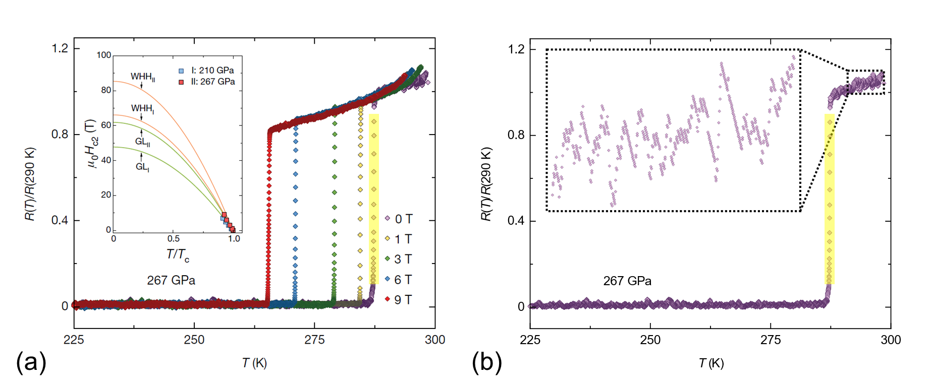
Before diving in the data behind the controversy – a short intro on super-conductivity is in place. As the name implies, a superconductor has zero resistance when the temperature drops below a certain critical value. One obvious way to identify superconductivity thus is to measure the resistance of the material as a function of temperature and look for a sudden drop to zero. The left panel in Figure 1 below shows some typical temperature-dependent resistance curves from the Nature paper, with the steep resistance drop upon cooling indicated by a blue arrow.

When a material is superconducting it will also push out external magnetic fields: a magnetic field trying to penetrate a superconductor will induce an ever-lasting current that generates the exact opposite magnetic field, perfectly cancelling it out. This is the mechanism behind the Meissner effect, the phenomenon that a superconducting material can float above a magnet (middle panel in Figure 1 above). These magnetic effects are seen as a more stringent test of superconductivity and hence the measurement of the so-called magnetic susceptibility of the material becomes important. Also this magnetic susceptibility should show a step-like jump at the critical temperature, with examples from the Nature paper shown in panel (c) of Figure 1.

The magnetic properties are hard to measure. The room-temperature superconductor is only superconducting at extreme pressures of several millions bar. These pressures can only be achieved in a diamond anvil press, shown in Figure 2 above, and then only in a tiny volume. The superconducting sample has the diameter of a hair (~80 μm), but then cut so short (~15 μm) that one is left with a flat, coin-shaped object. The magnetic properties are measured with coils (electromagnets) wrapped around the large anvil. As a result, one measures mostly anvil hardware and a tiny bit of superconducting material. The small signal from the superconductor is derived by subtracting a large ‘anvil’ background from the measured signal:
corrected = measured – background
The background in the equation above is exactly the one mentioned in the retraction: “the background subtractions applied to the raw data […] used a non-standard, user-defined procedure”.
The paper gets published and questioned
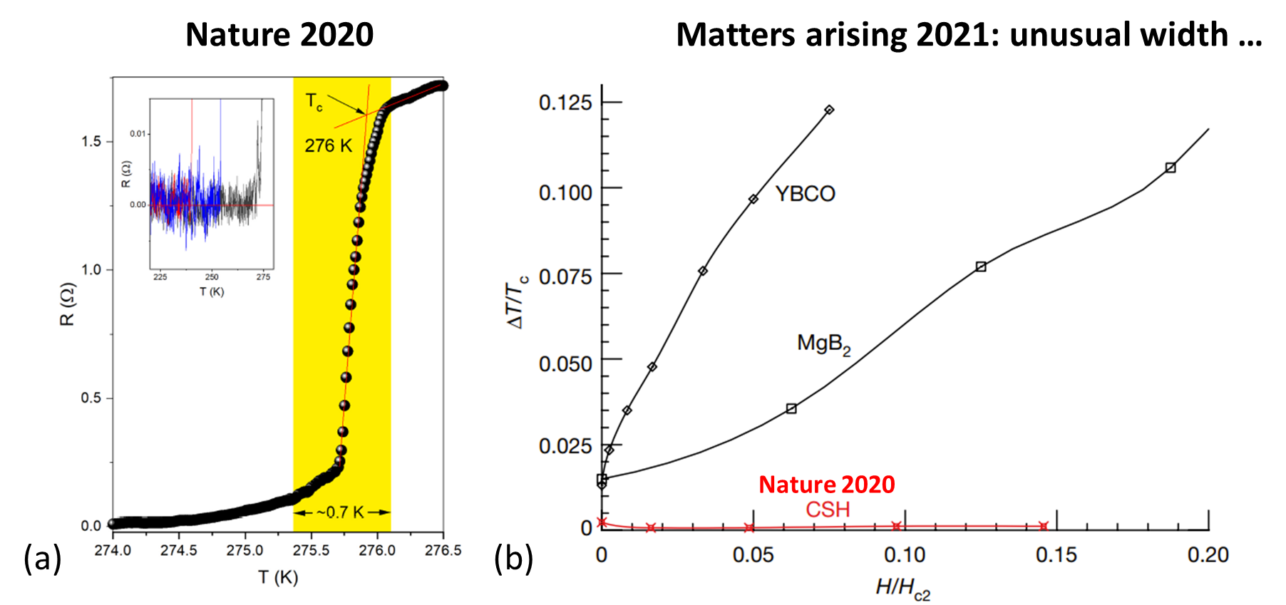
The room-temperature superconductivity article was published October 14th, 2020. Only six days later, Hirsch and Marsiglio submitted a ‘Matters arising’ comment to Nature. In it they question the extremely narrow widths of the superconducting resistance transitions, summarized in Figure 3 below. Its initial effect was limited, as it took 10 months to get published.
In addition, its main point was that the curious room-temperature superconductor showed a curiously sharp superconducting transition. And this might just as well be another surprise of the exotic material.
One month later Hirsch fires another shot by posting an arXiv pre-print that was rapidly accepted by Physica C, appearing online only two months after the Nature paper. In it he takes aim at the magnetic susceptibility data in both the Nature paper as well as the 2009 PRL paper mentioned earlier. The argument is again technical, but please hang on: our next stop will be plain fraud!
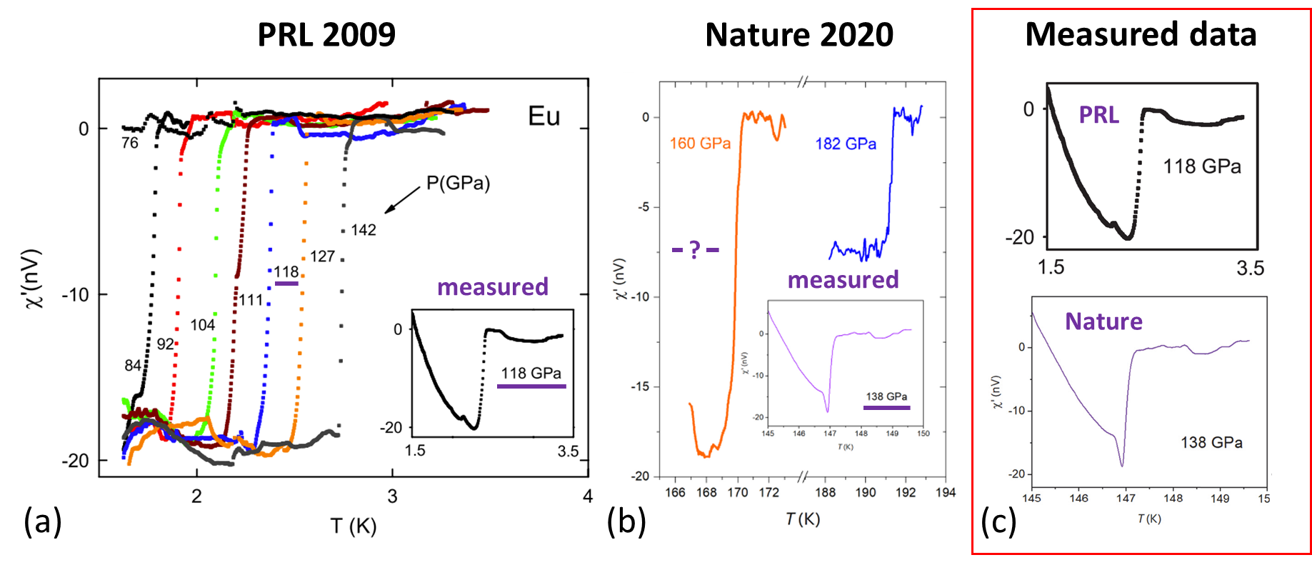
The PRL and Nature papers each show a single raw susceptibility measurement as an inset of a figure, see Figure 4(a) and (b) above. The measurement data in both papers looks very similar, panel (c), despite being measured on different materials having hugely different superconducting temperatures (2.5 K versus 147 K).
For the PRL paper also the corresponding background-corrected data was published, see the blue, step-like 118 GPa curve in Figure 4(a) above. This allows one to reconstruct the background: background = measured – corrected. Figure 5(a) below shows this background in red. It consists of an approximately linear part above Tc (solid orange line) and a strongly curved part below Tc (dotted orange line). The background is due to the diamond anvil and was said to be independently measured. It thus is expected to be independent of the superconducting transition, but curiously it features align with Tc.
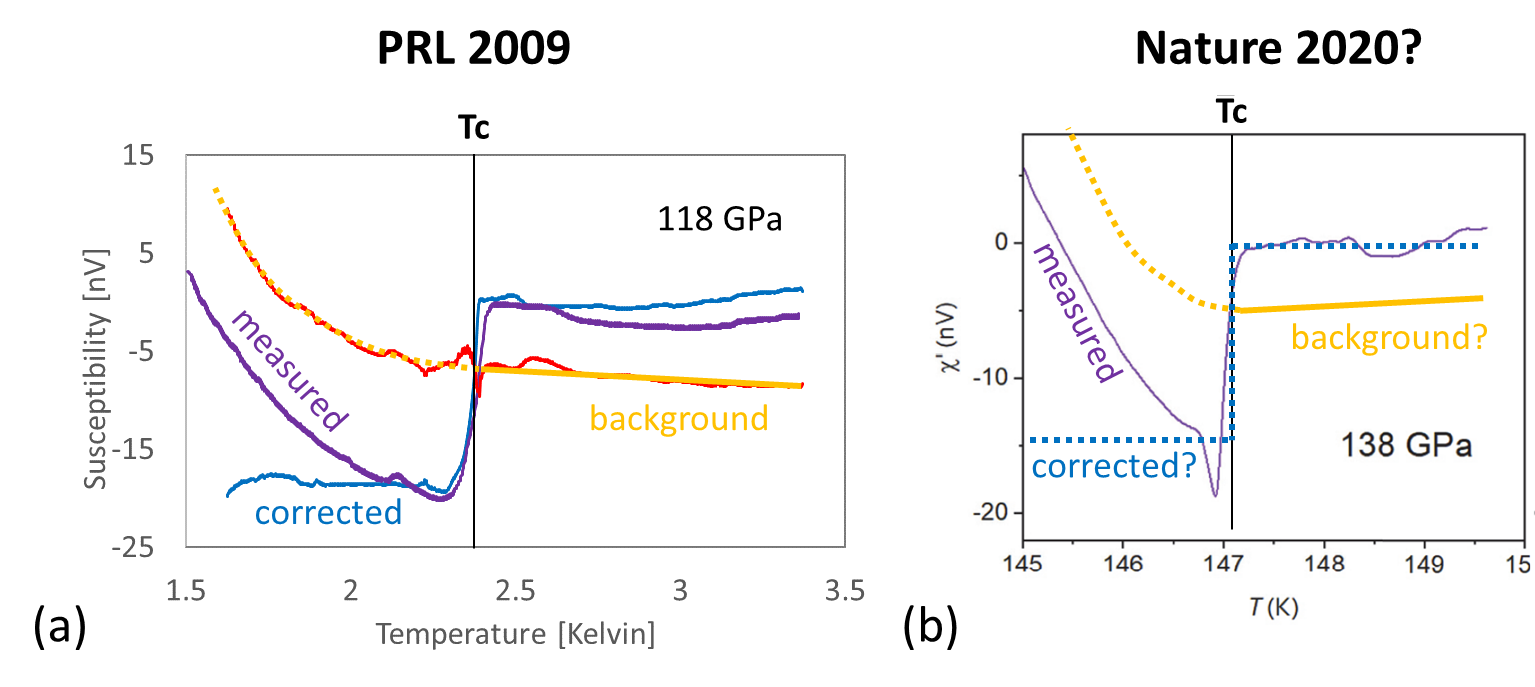
Intriguingly, the Nature paper does not show the matching corrected data. If the corrected data would also be step-like as the other published curves, then the supposed anvil background would again show a strongly curved low-temperature part that is linked to Tc, see Figure 5(b).
Based on the above Hirsch argued that the strongly curved parts in the measurement data are not due to background effects, but due to magnetic effects in the sample. And since this signature does not fit a superconducting transition, one is likely observing much more mundane magnetic effects. This would all be easy to check with access to the measured data. Hirsch asked, but no data was shared.
Fraud in the PRL paper
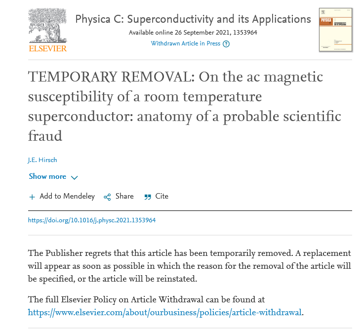
Fast forward to November 2021. Hirsch has finally received raw data, but only for the PRL paper. This took 8 months, many requests, and the threat of contacting the integrity office at the NSF funding agency. And he goes nuclear by publishing a paper titled “On the ac magnetic susceptibility of a room temperature superconductor: anatomy of a probable scientific fraud“. This title is an obvious lightning rod for defamation lawyers and it did not take long before the publisher invented a “TEMPORARY REMOVAL”. You can, however, still find the paper on Hirsch’s personal website.
The content happens to be a fatal shot at the PRL paper and another step towards the demise of the Nature paper.
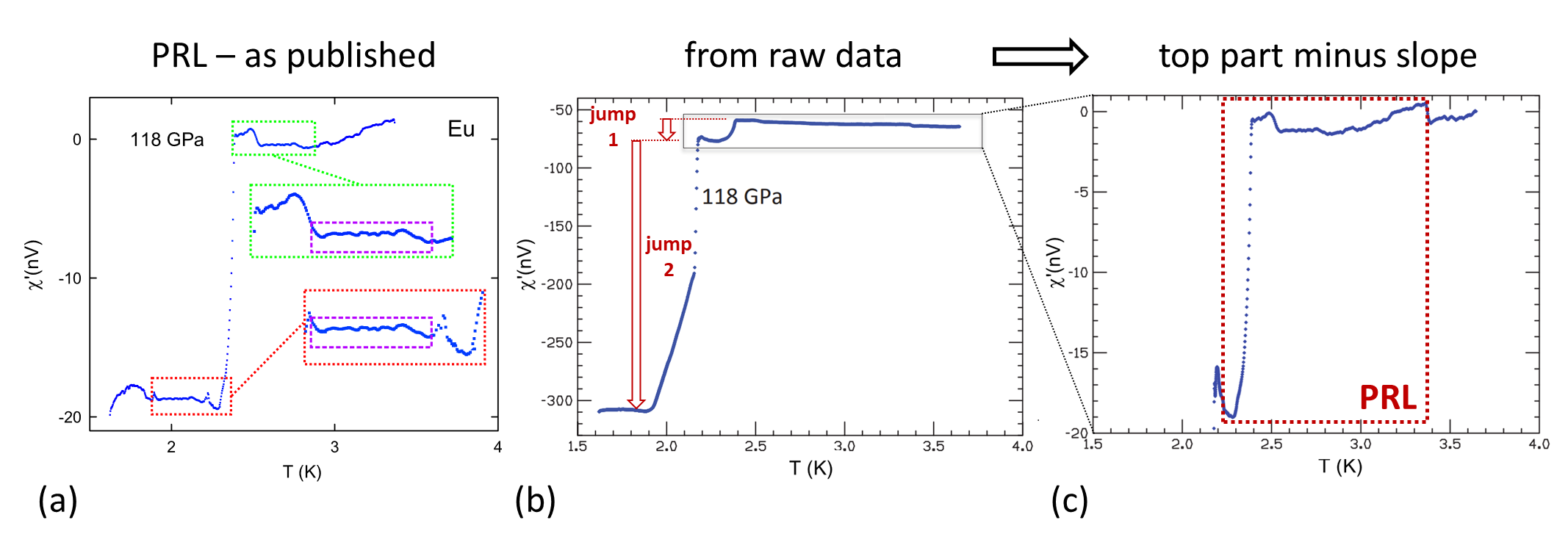
Let’s first start with some obvious fabrication in the 118 GPa data that we examined before. The as-published data is replotted in Figure 6(a) after digitally removing all other curves. Zooming in on the bottom and top parts, red and green rectangles, one can identify a large stretch of duplicated data inside the magenta rectangles. This is a clear sign of fabrication, plainly visible in the published results.
Using the shared data Hirsch tried to reconstruct the background-corrected curve, Figure 6(b) above. On first sight there is little resemblance with the published data in panel (a): the curve shows two jumps instead of one and the total step is more than 10x higher than that of the published curve. With the help of James Hamlin a connection was found: when only considering the upper part of the data (rectangular box) and after adding a linear term one obtains the curve in panel (c) above. The region enclosed by the red rectangle is identical to the high temperature part of the published PRL curve in panel (a). And we already found where a part of the low temperature data came from: fabrication by a copy-paste from the high temperature part.
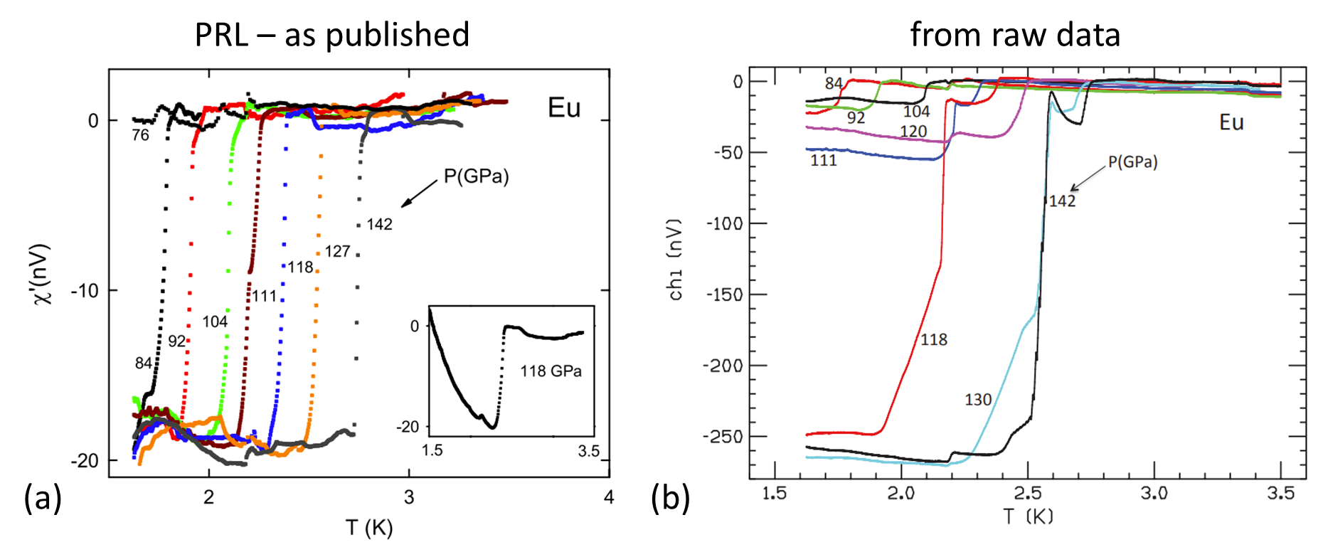
As you may have expected, the issues with the PRL paper were not confined to the 118 GPa data: the picture-perfect published curves reproduced in Figure 7(a) below only have a fleeting resemblance to those in panel (b) that were derived from the actual data. In short: the complete published susceptibility dataset had been fabricated.
In the Physica C paper mentioned earlier Hirsch questioned the very similar measurement data published in the PRL and the Nature studies (see Figures 4 & 5). By now it is clear that the PRL data was faked. Which obviously is not a good omen for the data of the Nature paper.
Mounting pressure
The ‘controversy’ initially did not gain much attention, despite the multiple critical papers published by Hirsch. This changed when August 2021, 10 (!) months after submission, his ‘Matters arising: Unusual width of …’ submission was published in Nature. Only one day later Science published a news article on it. Experts interviewed there still considered the data plausible and Dias explained he could not share data because he was “filing patent applications, so his lawyers have asked him to withhold the data for now“. Which is a completely bogus argument.
The ‘anatomy of a fraud’ paper caused another stir, with Science reporting on it October 2021. Dias is quoted there saying “Hirsch is a troll. We are not going to feed this troll” (by providing the data). Another month later the 2009 PRL paper is retracted by its authors. The retraction notice contains a very oblique nod to the fraud that has taken place: “In addition, an extensive reanalysis of the original raw data by one of the authors revealed that the susceptibility data presented in Fig. 2 were not accurately reported.” (emphasis mine). Hirsch is acknowledged for discussions.
By now the pressure on the Nature authors is mounting to share their experimental data. And they eventually did so in two batches.
In November 2021, a limited dataset was released as an arXiv pre-print. It only contained the measured data for four curves. As you may expect this did not stop Hirsch, who combined it with background-corrected data he digitized from the Nature paper to find concerns that I will spare you.
In December 2021 more data followed in an update to the pre-print, reporting both measured and background-corrected data for a larger number of measurements. The extra data was added as some 80 pages of images of tables.
Fraud in the Nature paper
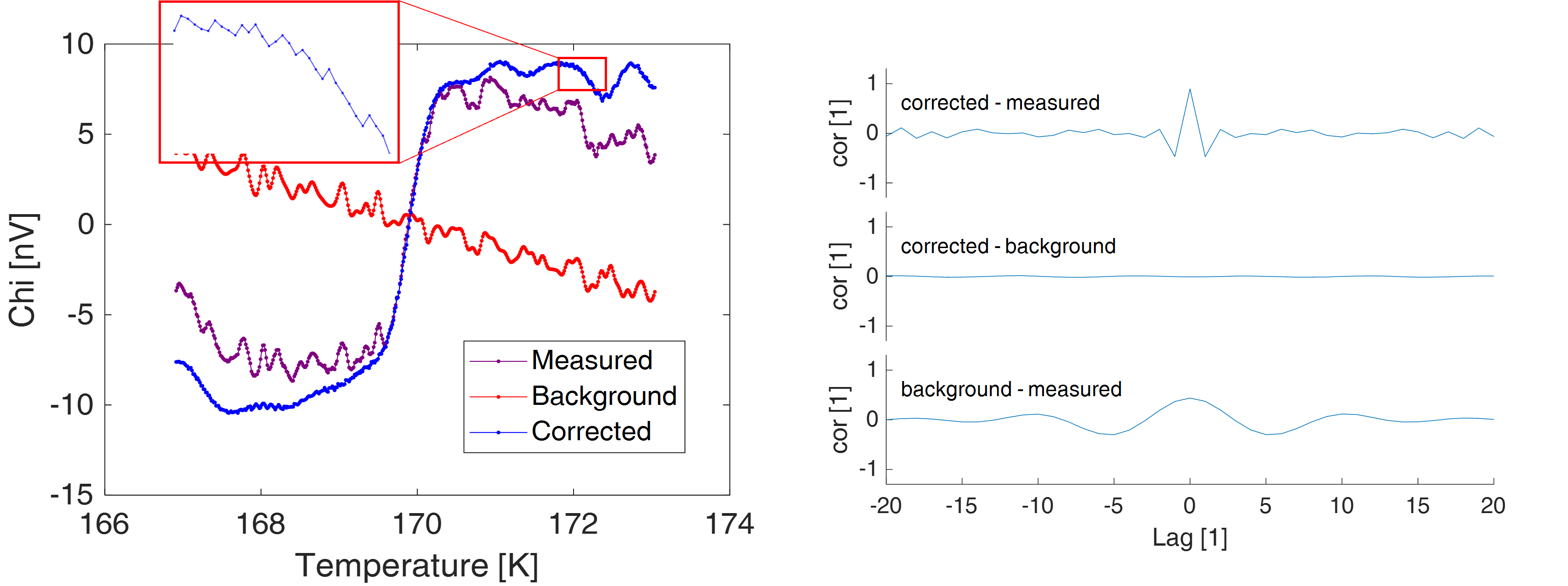
Hirsch teamed up with Dirk van der Marel, a (recently emeritus) professor of the University of Geneva in Switzerland. Together they published a short but scathing analysis of the measurement data on arXiv, January 2022. In their two page paper they focus on a single and truly odd dataset, reproduced in Figure (8) below.
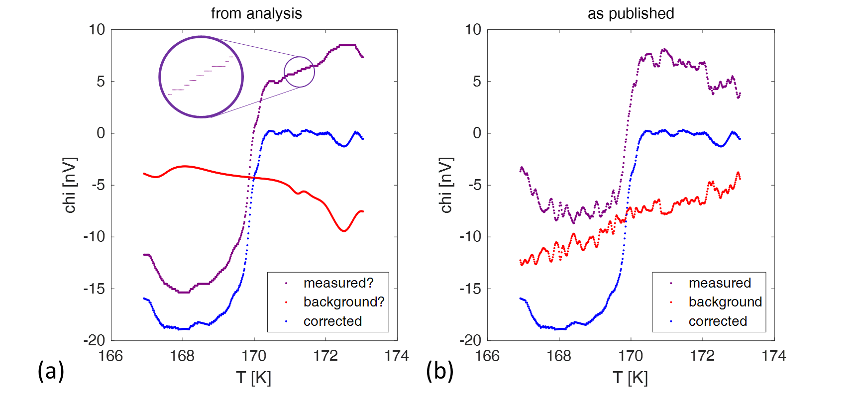
The inset in panel (a) shows the obviously wrong feature: the background-corrected data consists of an apparently smooth curve that at irregular intervals shows a large step. van der Marel removed all the steps using a procedure that is shown animated in the right panel. And he found that he was left with a perfectly smooth curve. In fact, the curve happened to be a mathematical function that can be used for smoothing (for the connoisseur: a 15 point cubic spline).
Puzzled, the critics guessed that maybe the authors had heavily smoothed the subtracted background measurement. This then leads to the identification shown in Fig. 9(a) below: a weirdly stepped measurement in purple and a noiseless background in red. Which, after subtraction, results in the ‘zig-zag’ corrected data in blue. However, the measured data and background published by the authors looked nothing like this, see panel (b).
Looking at the pathological data and its incompatibility with the given method, the critics state in their preprint:
“We conclude that the published data have been manipulated“.
The Nature authors strongly disagreed with that conclusion. Apart from sending a cease-and-desist letter, Dias and Salamat also offered a reply on arXiv 10 days later. Its abstract speaks of “a lack of scientific understanding” on the part of the critics. And its contents are a sublime example of moving goal posts and smoke & mirrors.
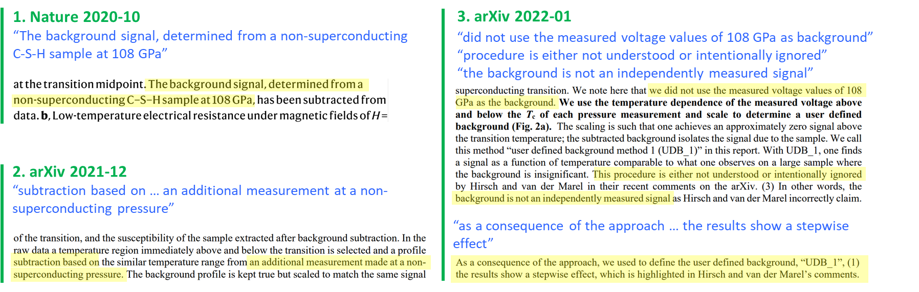
The 2020 Nature paper was very clear on the background subtraction method, see Fig. 10 above: the background is determined from a non-superconducting measurement at 108 GPa. Which is incidentally the same method that was used in the PRL paper. The text accompanying the 2021-12 arXiv data release is less crisp, but clearly states that the “subtraction (is) based on […] an additional measurement made at a non-superconducting pressure“.
In their January reply Dias and Salamat suddenly pull a joker card: “we did not use the measured voltages of 108 GPa as background” (emphasis mine). The authors then provide a short and faint sketch of a procedure, leaving out all the details needed for reproduction. It is actually reproduced in full in Fig. 10, but see also my comments here. Next follows a fully undeserved stab at their critics:
“This procedure is either not understood or intentionally ignored by Hirsch and van der Marel“.
And then the authors create a smoke screen by detailing two background procedures that could have been, but were not used. And to finish it off: “As a consequence of the [undocumented, -MvK] approach we used to define the user defined background, the results show a stepwise effect“.
The scientific look and the chutzpah with which the response was presented could certainly be enough to convince an editor. This left Hirsch and van der Marel with the daunting task of showing that the submitted data was fraudulent without having knowledge of the magical background procedure that was supposed to produce the ‘stepwise effect’. And they managed, even in a number of independent ways. For your comfort I will only show one, though.
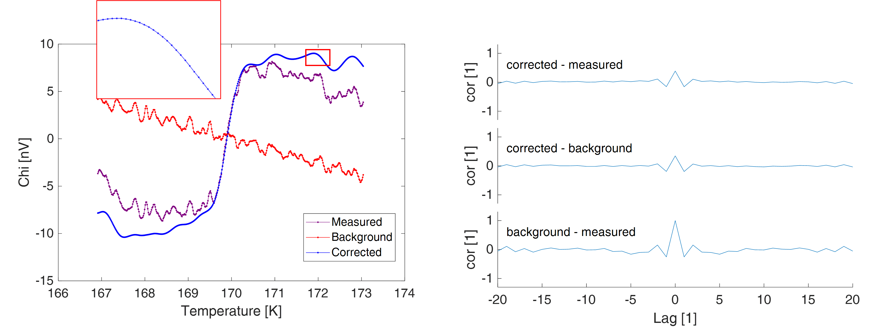
The corrected data is supposed to be related to the measured data and the background: corrected = measured – background. As a result, features in both the measured data as well as the background should leave an ‘imprint’ in the corrected data. This is exaggerated in Figure 10(a) below where the corrected data in blue shows the imprint of the smooth measurement in purple an the wiggly background in red.
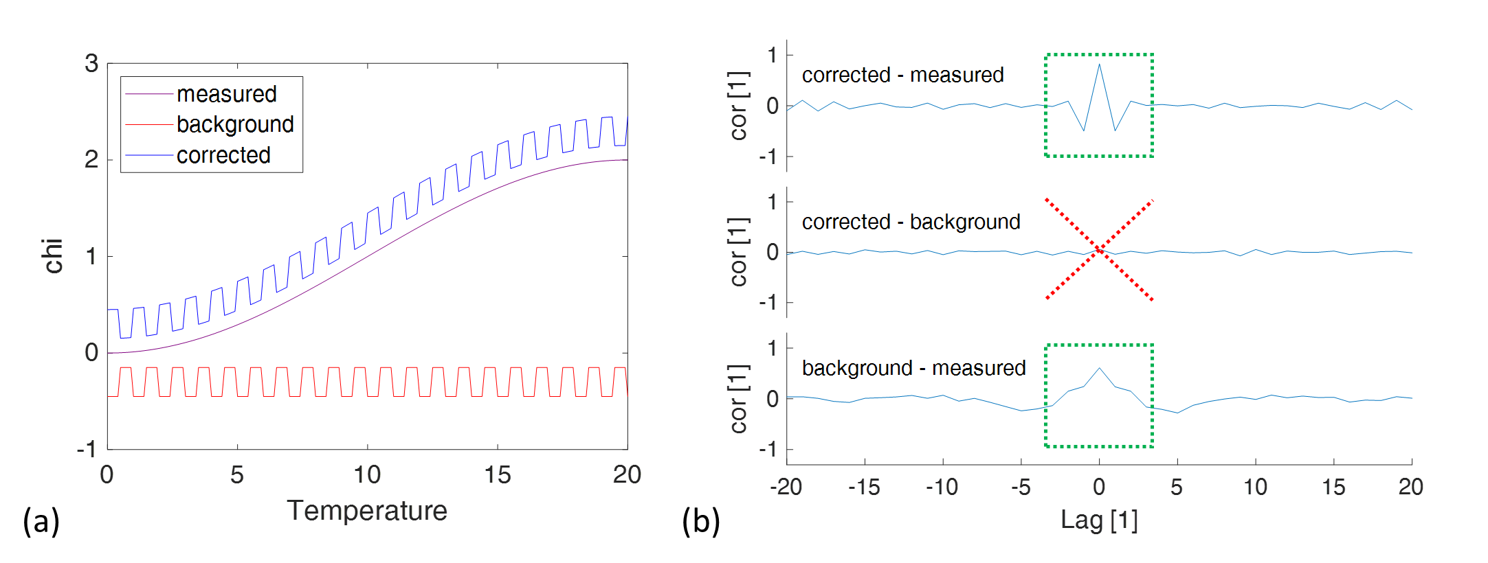
One can statistically tests for such imprints by looking at cross-correlations between datasets. These cross-correlations are shown in panel (b) for the 160 GPa dataset. When two datasets are correlated one will see a positive or negative peak at zero lag. This peak is missing for the correlation between the corrected data and the background (middle figure), plainly showing that the corrected data is unrelated to the supposedly subtracted background.
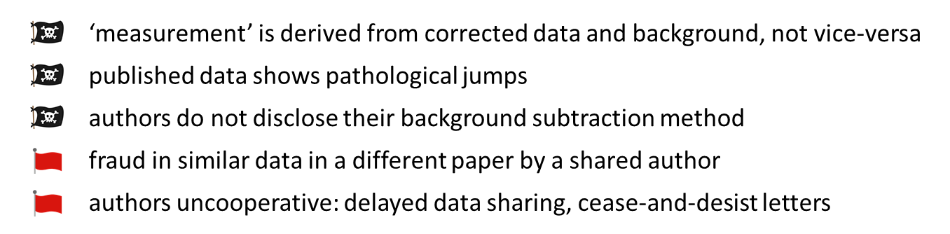
Instead, the measured data is found to be related to the background and corrected data. This result is only [see Reply to John] compatible with a completely different approach: measured = corrected + background. And that is fabrication… To top it off: the authors showed this to be the case for all published datasets.
By now the Nature paper has many black and red flags (first one less firm now, see Reply to John):
September 2022 Nature decided to retract the paper, with none of the authors agreeing. The retraction notice is fully unhelpful when one wants to know what is amiss:
“We have now established that some key data processing steps—namely, the background subtractions applied to the raw data used to generate the magnetic susceptibility plots in Fig. 2a and Extended Data Fig. 7d—used a non-standard, user-defined procedure. The details of the procedure were not specified in the paper and the validity of the background subtraction has subsequently been called into question”
Final thoughts
The lack of data sharing by challenged authors is a recurring issue, see e.g. this high-profile retraction and tweets by one of the whistleblowers. The papers invariably contain the ‘data available upon request’ statement. Natural sciences are about phenomena that can be reproduced under identical conditions. To make this possible, it is of crucial importance that scientific publications provide an accurate description of the methods of data acquisition and analysis, and of the data themselves. Journals, universities, and funding agencies should not accept the denial of data access.
The retraction notices of the PRL and Nature paper neither mention fraud nor misconduct. The Nature retraction states that the authors failed to report the “details of the (background-subtraction) procedure in the paper“. But fully neglects to mention that the authors refused to explain the method at all. These oblique and ‘positive’ notices are likely driven by the fear of legal action from the side of the authors. They are unhelpful in the valuation of the (de)published science and only provide limited discouragement to fraudulent authors.
It is astonishing and worrying that none of the nine authors took responsibility by agreeing with the retraction. This may be because money is involved. As the University of Rochester proudly mentions, the authors founded a start-up company, Unearthly Materials. You can even license their patented IP at the university’s URventures.
I do, however, like a more cynical explanation for their endorsement of fraud. The authors may simply fear that an admission will negatively affect their hirsch-index…
Authors’ explanation of the background subtraction procedure
Below the authors’ full explanation of the background subtraction procedure:
“We use the temperature dependence of the measured voltage above and below the Tc of each pressure measurement and scale to determine a user defined background (Fig. 2a). The scaling is such that one achieves an approximately zero signal above the transition temperature; the subtracted background isolates the signal due to the sample. We call this method “user defined background method 1 (UDB_1)” in this report. With UDB_1, one finds a signal as a function of temperature comparable to what one observes on a large sample where
(arXiv 2021-01)
the background is insignificant. This procedure is either not understood or intentionally ignored by Hirsch and van der Marel in their recent comments on the arXiv. (3) In other words, the background is not an independently measured signal”
The explanation is accompanied by this figure:
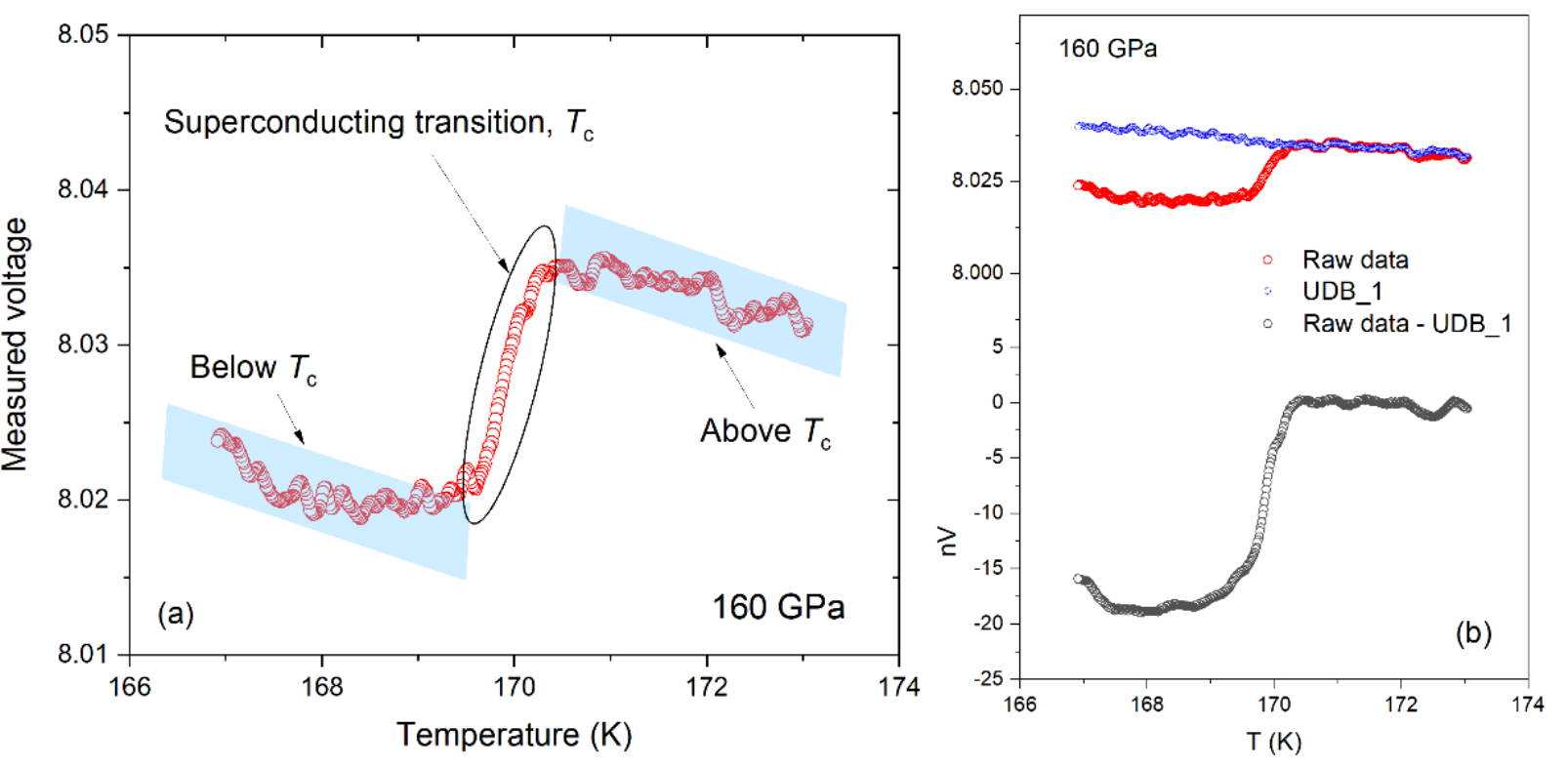
highlighted in blue are used as part of the UDB_1. (b) Measured voltage from the
susceptibility measurement explained in experimental details section in Ref. 1 and 2 for 160
GPa. Raw data (red), UDB_1 (blue) and raw data – UDB_1 (black).
The authors explain that they use the measured data above and below Tc (shaded in blue in the figure) to determine the background. They scale this data to obtain the user-defined background. The scaling method is undefined, except that it “is such that one achieves an approximately zero signal above the transition temperature”.
The most obvious way to achieve a ‘zero signal above the transition temperature’ is to apply no scaling to the ‘above Tc’ part: subtracting ‘above Tc’ from itself would result in the desired zero signal… It is also not explained how one would ‘scale’ or otherwise treat the ‘below Tc’ part.
In the right panel of the figure the authors show their background in blue. It shows interesting wiggles, even in the region between the shaded areas. It is left completely unexplained where the background data in this region comes from. The authors do state that “the background is not an independently measured signal”. So somehow the authors are able to accurately derive a background from the steep transition region in the measured data.
The published corrected data turns out to be the sum of a cubic spline function and a strangely stepped signal, see Figure 8. The authors nowhere mention smoothing or splines in their explanation. Yet they are perfectly happy stating that “the artifacts … are due to the user defined background subtraction method”.
The authors are hiding far more than they are revealing in their explanation of the background determination.
Update 2022-10-21
James Hamlin published a pre-print analyzing the resistance data in the Nature paper. The issues will by now sound familiar.
In the left panel of the figure below I have reproduced Fig. 3b from the Nature paper. Its resistance versus temperature curves all show an unusually narrow step when the material transitions from superconducting to normal, a surprising result that was pointed out by Hirsch in his Matters Arising comment. The odd nature of the data itself went, however, unnoticed.
The right panel shows the same figure after digitally removing all but the 0 T curve (highlighted yellow). The inset is a zoom-in of the data in the top-right. It can be seen that the data looks familiarly weird: the measurement is made up of stretches of nearly linearly decreasing resistance, with at irregular intervals vertical jumps. This is all very much like the susceptibility data shown in Fig. 8 of this post.
Hamlin also took the next step, removing the jumps to find whether also here the data was the sum of a smooth and a stepped curve. And no disappointment here, see the figure below: the high temperature part of the published data in red consists of a steeply dropping ‘smooth part’ in orange added to a steeply rising ‘digitized part’ in blue. The likeness to the susceptibility data shown in the right panel is evident, including the equal-sized steps (x N) in the respectively ‘digitized’ and ‘measured?’ parts.

The authors gave the below explanation for the “stepwise effect” in the susceptibility data:
As a consequence of the approach, we used to define the user defined background, “UDB_1”, (1) the results show a stepwise effect, which is highlighted in Hirsch and van der Marel’s comments.
arXiv:2201.11883v1
This ‘explanation’ cannot hold for the resistance data; the resistance measurement is much simpler and no background subtraction procedure is needed. And, importantly, no such procedure is specified in the paper. Note that there is no overlap in measurement equipment between the susceptibility and resistance measurements that can explain the shared ‘pathology’.
As a result, the list of concerns has further grown:

Reply to John
Based on your questions I decided to look a bit closer at the cross-correlations in Fig. 10b. And yes, I can device a scenario where the background is derived from the measurement and no correlation is seen between background and corrected curve.
The narrow width of the “corrected to measured” cross-correlation shows that it is mostly driven by higher frequencies. This can be visualized by high-pass filtering the corrected and measured data:
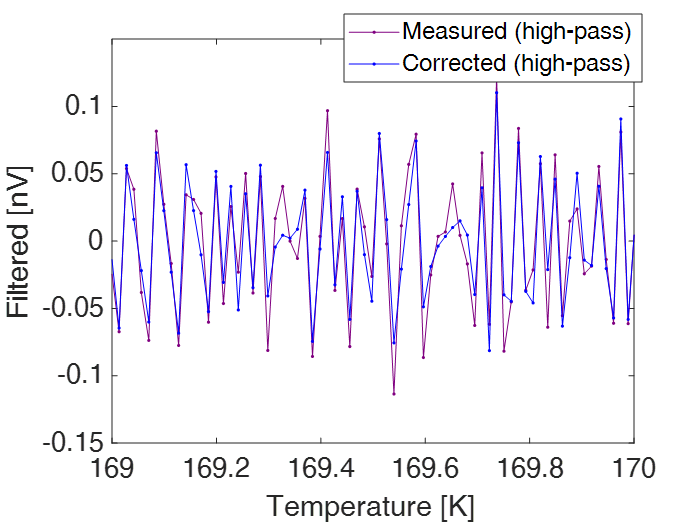
The high-frequency part of the corrected and measured curves are very alike. And the ‘sawtooth pattern’ in both is very likely related to the ’12 point spline plus digital steps’ deconstruction made above (but then filtered quite a bit). Assuming ‘corrected = measured – background’, this means that the deduced background did not remove the high frequencies. The high-frequency part of the background is actually the difference between the curves in the figure above. And thus small.
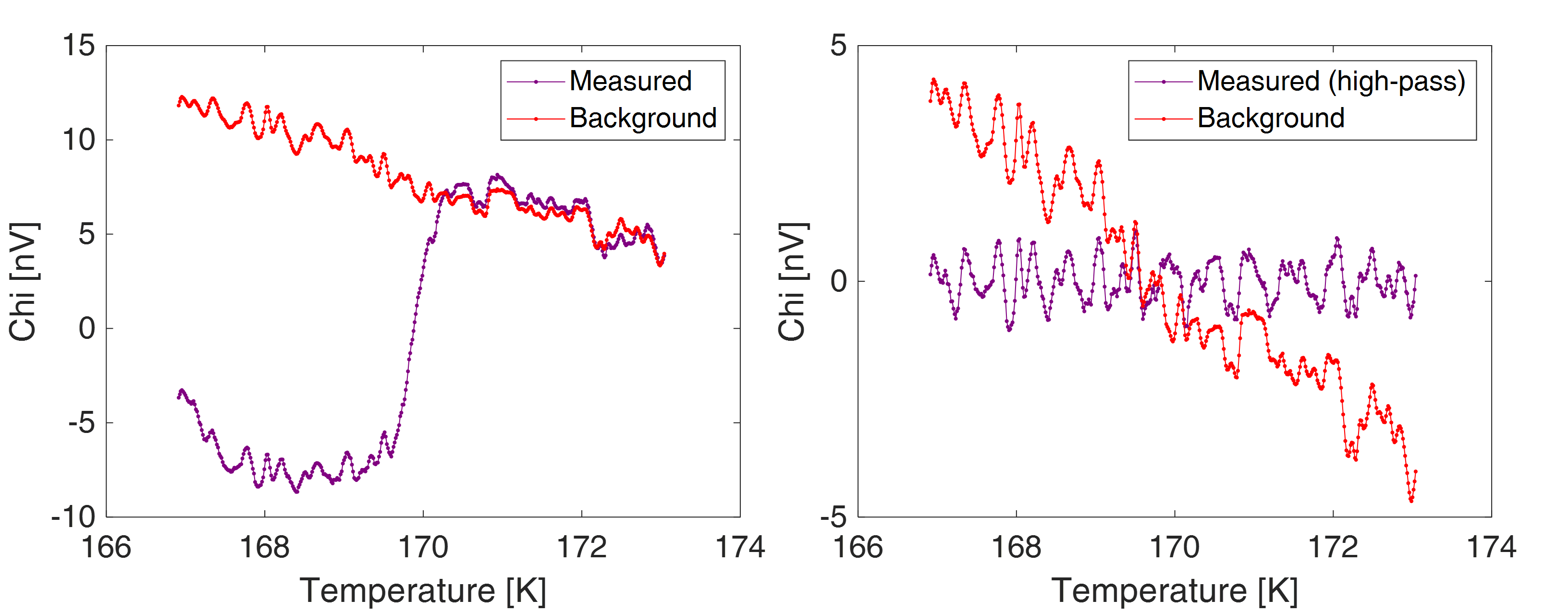
The background is both visually as well as in the explanation of the authors related to the measurement. In the left panel above I plot the 166 GPa measurement and background curves, shifted vertically to make them nicely overlap. The authors never explained how they got this background that is similar but not identical to the measured curve. And even has detail in the sharp transition around 170 K.
One conjecture could be again high pass filtering. In the right panel I tried this with some optimized cut-off value. The step is gone and the wiggles look somewhat like the published background curve. But together with the step also the ‘linear’ slope is removed: the linear part depends on the now-removed low-frequency components.

In the figure above I have simply removed the linear term from the published background curve (in red) to ease comparison. And compare it in the left panel to high-pass filtered measured curve (purple). The purple curve has some similarity, but is also more ‘jagged’. That is in line with our earlier observation: the published background curve lacks high-frequency components. In the right panel I bandpass filter the measured curve; apart from removing the low frequencies (step, slope), I also remove high frequencies. This results in a visually similar curve.
So in the above I cooked up one way to get a similar-looking background curve: bandpass filter the measured data and subsequently add a linear term to correct for some undesired slope in the measured data. The measured, background, and corrected curves are shown in the panel left below. The corrected curve even shows some steps as our background subtraction effectively removes a mid-frequency range and thus brings forward high frequencies. The right panel shows correlations. And the corrected curve is not correlated to the background, despite its ‘corrected = measured – background’ history. This is, however, not only related to subtracting a ‘modified version’ of the measurement from itself (and by that cancelling noise/similarities).
In the figure below I do not remove the high frequencies from the background signal (highpass instead of bandpass filtering). As a result the corrected curve is now very smooth as most of its high frequencies are ‘subtracted’ (left panel, inset). Its 2nd derivative (that we use for the correlation and that brings out ‘noise’) still shows some of the original features as (using this specific series of steps…) the high frequencies are not fully canceled (used a default 60 dB attenuation filter). And now all three curves are correlated with each other (right panel).
So the van der Marel conclusion is most correct: the published data is not compatible with “corrected = measured – background” when ‘measured’ and ‘background’ are both measurements. And it is compatible with “measured = corrected + background”. And, importantly, we cannot say what the author’s method would have yielded as it is not shared.
The above shows that there are scenarios where “corrected = measured – background” results in no visible correlation between corrected and background when the background is derived from the measurement using bandpass filtering. This thus is a correction on the too strong statement I made earlier.
Note that this does not decrease my suspicion against the paper. The above is still compatible with measured = corrected + background, with some made-up background containing mostly lower frequency noise (longer undulations). And it still defies belief that subtracting a ‘however-derived’ background from a measurement results in a corrected curve that is the sum of a 12 point spline and some stepped curve. I am also pretty sure that the high-pass filtering of the measured data (topmost figure in this section) shows that the spline was already present in the ‘measured’ data. And that obviously should not be.
Reply to John 2
- “Was the background in the red curve in Fig 9b provided by the authors?”
In the most strict sense the authors only provided the measured and corrected curves, see https://arxiv.org/ftp/arxiv/papers/2111/2111.15017.pdf and the screenshot below. With the 11 decimals or more in the table and the ‘corrected = measured – background’ relation not in question, the background used by the authors is trivially found by subtraction.
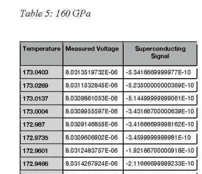
2. “If you remove the discontinuities between the “odd steps” like done by Van der Marel, do you find a continuous curve similar to the one shown in Fig. 8b or 9a (red)?”
If that would be the case, then my background would have been identical to that of the authors. There is not much wiggle room in an ‘a = b – c’ equation.
What I think is a plausible scenario is that the authors generated the measured data by adding a made-up wiggly background curve to the published corrected values. The made-up wiggly background curve has little information at high frequencies, and, apart from its slope, also little information at low frequencies. And hence by bandpass filtering the (generated) ‘measured’ data and adding a slope I can partially reconstruct the background. And as a result I can partially reproduce the odd features seen in the published corrected curve: ‘digitization’ steps and smooth sections, see below. This explanation anyway makes much more sense than having a background-determination procedure that transforms a wiggly measurement curve in the sum of a 12 point spline and a stepped function.
PS by L. Schneider
The new Nature retraction may be Hirsch’s third scoop. Also Ashkan Salamat, once a hero of his Las Vegas university, had another retraction, in 2016 already:
Mario Santoro , Federico A. Gorelli , Roberto Bini , Ashkan Salamat , Gaston Garbarino , Claire Levelut , Olivier Cambon , Julien Haines Carbon enters silica forming a cristobalite-type CO2–SiO2 solid solution Nature Communications (2014) doi: 10.1038/ncomms4761
That retraction was presented as an honest mistake by honest scientists which Salamat is definitely not.
Also, PubPeer user Thallarcha lechrioleuca found this, by Salamat as PhD student:
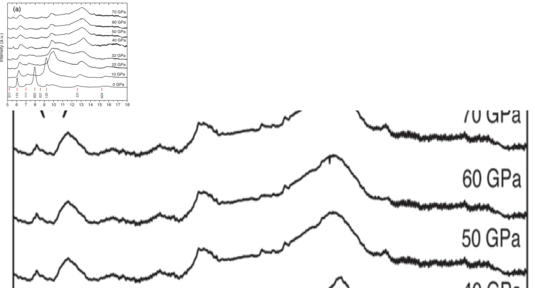
Ashkan Salamat , Katherine Woodhead , S. Imran U. Shah , Andrew L. Hector, Paul F. McMillan Synthesis of U3Se5 and U3Te5 type polymorphs of Ta3N5 by combining high pressure–temperature pathways with a chemical precursor approach Chemical communications (2014) doi: 10.1039/c4cc05147e
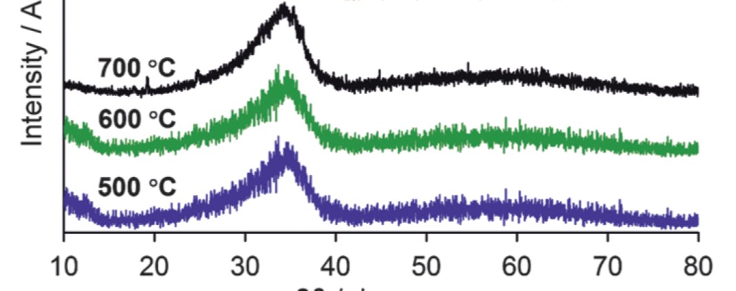
It’s called fake spectra. And this, more fake spectra:
Ashkan Salamat, Malek Deifallah , Raul Quesada Cabrera , Furio Corà , Paul F. McMillan Identification of new pillared-layered carbon nitride materials at high pressure Scientific Reports (2013) doi: 10.1038/srep02122
The last author, the UCL professor Paul McMillan, died in February 2022. He can’t defend himself now from the damage his PhD student Salamat caused to his reputation.
Salamat’s career might be circling the drain now, he deleted his lab’s website. But Dias may be in a better position. A year ago, University of Rochester reported “a $1.6 million grant from the Gordan and Betty Moore Foundation to support his groundbreaking efforts to create viable superconducting materials“, plus “a $794,000 National Science Foundation (NSF) CAREER award to fund his efforts to instead create ternary (three-component) and quaternary (four-component) compounds with the right chemical structure and chemical bonding of materials to remain superconducting at ambient pressures“. Plus the cash raised from investors for Dias’ Rochester start-up Unearthly Materials. The University wouldn’t want to be asked to return that money.
Let’s conclude with Dias’ own words:
“So much to say to explain the level of hardship. I can write a book about it. I never complained about any of the difficulties that I had to go through. I always took that as a part of the journey we all have to go through. Who we are going to be is defined by how we dealt with those difficulties.”
This greedy cheater sent lawyers to threaten his peers when first “difficulties” arose. That’s how he will be defined.
I thank all my donors for supporting my journalism. You can be one of them!
Make a one-time donation:
I thank all my donors for supporting my journalism. You can be one of them!
Make a monthly donation:
Choose an amount
Or enter a custom amount
Your contribution is appreciated.
Your contribution is appreciated.


_-_2.jpg)
Two considerations:
1) Dr Dias is always wearing the same pullover and shirt in all the photos, always the same outfit like super heroes!
2) if a paper about the “Holy Graal” of superconductivity gets published in Nature, one would expect the greatest standard of scrutinity, right? Not at all: Hirsch found major issues in no time, and submitted a letter to Nature to expose the fraud six days later the paper was accepted. Take home message: you can imagine, dear reader, what gets through in middle-level (although respected) journals on niche topics in all fields.
LikeLike
Possible explanation for point 1): Maybe Mathew is just using his famous copy+paste techniques on Ranga’s photos 🙂
LikeLiked by 1 person
The retracted Nature paper acknowledges support from NSF grant DMR-1809649. NSF policy states “Investigators are expected to share with other researchers, at no more than incremental cost and within a reasonable time, the primary data, samples, physical collections and other supporting materials created or gathered in the course of work under NSF grants. Grantees are expected to encourage and facilitate such sharing.” There is no excuse I can see for not providing data upon request, including the (bogus) protection of intellectual property. See: https://www.nsf.gov/bfa/dias/policy/dmp.jsp
LikeLike
At the very least, we can agree to refer to “a non-standard, user-defined procedure” as a Dias. Not a Nobel, but something for his efforts.
LikeLike
Nice piece and entirely accurate. Thank you Maarten.
To KM: you are being fooled by the wording “are expected to share”, as I was. This is from the horse’s mouth, NSF-OIG (DMR is Division of Materials Research):
“NSF data sharing policy creates an expectation, but not a requirement, for PIs to share data. Each division implements this policy through Data Management Plans that are submitted with each proposal. DMR’s guidance reiterates NSF’s expectation and does not make it a requirement. The Data Management Plan for this grant states only that “There are a wide variety of formats available… to facilitate data sharing” but nothing that would extend sharing data beyond members of the group.”
LikeLiked by 1 person
Thank you. That is… disappointing.
LikeLike
A quick question for you, Jorge:
Now that it has been shown that the ACS and resistivity data have been heavily engineered (for lack of a better term), what do you make of the situation? For example, do you think there were probably hints of superconductivity, and then they just massaged the data to make it look better?
A question for the authors or the Nature paper:
If it was Mathew that manipulated the ACS data, who measured and manipulated the resistivity data?
LikeLike
I assume you are referring to arXiv:2210.10766 by Hamlin on resistance data, very interesting. The 9 authors of the Nature paper, that unanimously disagreed with the retraction, have a lot to explain.
LikeLike
I want add my compliments to those of Jorge. This is an excellent description by an author with a deep understanding of the technical aspects. Figure 8b is amazing.
I like to put in my 0.02 CHF on the issue of open data. This has been subject of heated debates in the Swiss science community a few years ago, when it started be introduced. Defining precise rules as to the exact format and contents of the data that should be published depends strongly on field, experiment and/or theory, so the question is how to define those rules if at all, and who should be in charge of that. Not all scientific papers depend on external funding, yet providing open data is important (to give a recent example written with Jorge Hirsch: https://doi.org/10.1142/S0217979223750012 , open data in https://doi.org/10/gqmhjh). I think that scientific journals should play a pro-active role here: A scientific paper in a peer reviewed journal should be accompanied with the data set at the moment of submission. The referees can tell if the paper is adequately substantiated with the experimental or theoretical data, and can ask for complementary information in the same way as they often do for the contents of the paper. This data set should then be published on-line, ideally by the publisher, simultaneously with the paper.
LikeLiked by 1 person
Compliments to all of you who put up a so long and uneven fight till success.
I would add 0.02 CHF on the issue of open peer review, it is as important as the data itself. It would be interesting to know the reviews this paper had for publication.
LikeLike
This paper has more than 350 citations for about 2 years. And what should be done with all these citing papers (and in general for any retracted paper)?!
Grants, impact factor (IF) and h-index has created the perfect medium for fraudsters. First thing journal editors look in a manuscript is the h-index of the principal investigator (PI), which merely shows if he/she belongs to a citation cartel, a term coined by George Frank in 1999, https://www.science.org/doi/full/10.1126/science.286.5437.53. If that’s the case, then reviews most probably by members of the citation cartel are written and the manuscript gets easily published. Everybody is a winner here, authors get a publication, reviewers get several citations and the paper will get also a decent number of citations boosting the impact factor of the journal, meaning more funds for the journal and the editorial staff.
But if the PI does not belong to a citation cartel, i.e. has low h-index, then immediate rejection takes place in most cases with a similar sentence in the reply from the editorial staff:
“We believe that the main results with this work is somehow insufficiently impacting and we thank the authors for their interest in publishing with us.”
Bottom line is not about science, it is about business, IF and h-index, (almost) nobody cares about true science, even universities, research institutes and governments. This is the reason a faulty paper takes so much effort to be retracted, if retracted at all, and its authors almost always to escape justice despite there is special law for such cases. All these have been countless times written in this blog by the owner and guest authors, I have just summarized them in short.
Personally, did not expect fraud in science to be so en masse but thanks to this blog and my experience, I need to correct my estimation for the 3rd time…
LikeLike
Derrick, thanks for pointing out Hamlin’s arXiv paper on the resistance data! I added an ‘update’ section describing his finds.
LikeLike
Sure thing! I’m no longer in academia, but I’ve enjoyed watching from the sidelines. Thank you for writing the article – it must’ve taken a lot of time to compile everything. It’s a bit of a shame that people like you, Jorge, James, Dirk, and others have had to spend so much time digging into this, but I’m glad you did.
Looking forward to hearing some responses from Ash and Ranga! Seems like they have plenty of explaining to do… to the science community, and to their investors.
LikeLike
sorry, i don’t understand. The corrected signal is obtained by removing the background from the measured signal. Therefore, ideally, the corrected signal should not be correlated with the background. Are you suggesting that, in practice, the subtraction is not perfect and therefore there should be a residual correlation?
LikeLike
Hello John,
The corrected signal is indeed obtained by removing the background from the measured signal:
corrected = measured – background
The subtraction process actually creates the correlation between ‘corrected’ and both ‘measured’ and ‘background’. I tried to visualize that in Fig. 10(a) where the corrected curve in blue shows the wiggles of the background in red and the ‘sine’ of the measured curve in purple. Creating a correlation between the corrected curve and the measured and background curves.
In a more practical case the measured and background curves are based on measurements with noise. When substracting these two to get the corrected curve the (uncorrelated) noise does not cancel. Instead, the noise in the corrected curve is higher (e.g. RMS_corrected^2 = RMS_measured^2 + RMS_background^2). And the noise (and signal) in the corrected curve then is correlated with that of the measured and background curves. I showed the correlations for the 2nd derivative of the measurements, so focusing mostly on noise.
The conclusions of van der Marel in https://www.worldscientific.com/doi/10.1142/S0217979223750012 (page 22-) are most correct. They state that the published result is incompatible with ‘corrected = measured – background’ where ‘measured’ and ‘background’ are separate measurements with their own noise (the background procedure as published). And that the result is compatible with ‘measured = corrected + background’. And that they cannot say what the updated background subtraction procedure of Dias et al. would yield, as the authors have not specified that procedure.
So there is a risk that due to lack of imagination there may be a subtraction procedure that results in an insignificant correlation between corrected and background measurement.
In https://arxiv.org/abs/2201.11883v1 and reproduced in this post under “Author’s explanation of the background subtraction method” the authors spend a few words on their background determination. They suggest it is based on the measurement itself. Optimistically this is in line with the correlation between ‘measured’ and ‘background’ as ‘background’ is apparently derived from ‘measured’. It is however completely unclear how this would result in a background as in Fig. 9b. And why subtracting this background leaves no correlation between ‘corrected’ and ‘background’. Or why the corrected curve then shows funny steps that somehow related to a spline function.
LikeLike
Thanks Maarten very much. If I understood correctly, the background in the Nature paper was created from the data itself and therefore contains, by design, all those little bumps and wiggles (noise?) that are in the measured data. It follows that, by construction, the “noise” in the background is the same noise that is in the measured data. Therefore they are not uncorrelated (as you stated in your reply). For instance, if I treat your blue curve (in the example you provided in Fig. 10a) as the measured signal and I extract a background from it given just by using the grooves in the blue curve then I end up with a background that looks like the red curve shown in Fig, 10, Then when I subtract this fabricated background (red) from the measured signal (blue curve), I will get a smooth curve without grooves that has no correlation with the background (the grooves). In this case the background subtraction leads to a corrected signal that has no correlations with the background. Sorry, I am not well versed in statistical properties of these kind of measurement and I may be missing something very fundamental. Apologies if that is the case.
LikeLike
Hello John,
See https://forbetterscience.com/2022/10/12/anatomy-of-a-retraction-2-superconductive-fraud/#replytojohn.
Yes, when deriving the background from the measurement there are scenarios that will result in no correlation between the corrected curve and the background. I did not do extensive checking, just played a bit with bandpass filtering of the measured signal to derive a background. And found a scenario that looked a bit like the published data and did not show a corrected-background correlaton.
Best regards,
Maarten
LikeLike
Thanks Maarten for looking into this. A clarification question: was the background in the red curve in Fig 9b provided by the authors? Couldn’t quite understand if the authors provided the background or if it was extracted from measured-corrected. If the latter, then isn’t the right “equation” to analyze given by background=measured – corrected? Also, with regard to your new analysis (reply to me) where you reconstruct a background from the measured data that does not leave an imprint, you show an inset in the figure with the “odd” steps. If you remove the discontinuities between the “odd steps” like done by Van der Marel, do you find a continuous curve similar to the one shown in Fig. 8b or 9a (red)?
LikeLike
See ‘John 2’!
LikeLike
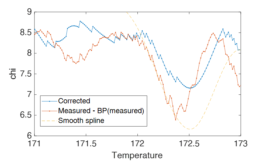
Dear Maarten. I was just reading about this story again and I have a follow up question. The authors claim that the artifacts in your Fig. 8a were introduced by the background UDB_1. As you indicated, these artifacts come from the 15p cubic spline shown in Fig. 8b. If the authors are right, there shouldn’t be any correlation between
the raw data and the cubic spline in 8b. Instead, the cubic spline should only be
correlated to the background UDB_1. Did you check for cross correlations between raw data and cubic spline, and correlations between background and cubic spline? Obviously there should not be any correlation between the raw data and the cubic spline if the raw data is indeed raw data.
LikeLike
Hello John,
The claim “As a consequence of the approach, we used to define the user defined background, “UDB_1”, (1) the results show a stepwise effect, which is highlighted in Hirsch and van der Marel’s comments” comes from https://arxiv.org/vc/arxiv/papers/2201/2201.11883v1.pdf (page 5).
The above is blaming an unphysical outcome on an undisclosed background determination method. While it is obvious that writing down how the UDB_1 method should not take more than a napkin and would solve everything, the authors ‘choose’ not to do that. Note that at the time of their response van der Marel et al. had not yet published/found that the smooth part was a perfect cubic spline curve. The authors thus do not comment on that anomaly.
With respect to your question on the correlation between the smooth spline curve and the author’s data: no, I did not try to make these correlations. You can have a look at Fig. 5 of van der Marel’s arXiv paper https://arxiv.org/pdf/2201.07686v7.pdf. There the smooth curve is plotted together with the measured chi_mv data and ‘UDB_1’ (chi_bg). Showing how dissimilar these are.
The smooth curve is obviously smooth and only has very low-frequency components. In Fig. 5b you can see some wide features at 167.5 K, 171.2 K, and 172.5 K. There is nothing in chi_mv in Fig. 5a that correlates with these features.
LikeLike
Another pubpeer comment: https://pubpeer.com/publications/F342DD2D2E72E5E2FD507089562B94
LikeLike
Interesting, it is not getting better. There are obvious common authors on the papers. It still strikes me that this happens in papers with so many authors, many of which contributed experimentally.
There is also https://pubpeer.com/publications/69EDBAECD50F31B051ECECCD1DF346#1. May be a minor oddity, though.
LikeLike
Publishing integrity quiz:
Your journal retracted a paper because, after post-publication peer review, you found it did not meet your quality standards. More specifically, there were signs of data fabrication. All authors object to the retraction, showing that they their quality standards differ from that of your journal.
Would you accept another paper from the same group of authors?
This publisher says: yes, sure! https://www.nature.com/articles/s41586-023-05742-0
The more interesting story featuring Hirsch: https://www.quantamagazine.org/room-temperature-superconductor-discovery-meets-with-resistance-20230308/
For technological progress I hope the results hold up. Personally I think Dias does not disserve the (possible) success after not owing up to his previous mess(es).
LikeLike
The timeline must also be pretty unique. The breakthrough superconductivity paper of this post was retracted 26 September 2022. The authors had already submitted their new Nature breaktrhough manuscript 26 April 2022. So whilst the one paper superconductivity paper was being retracted, the other was being reviewed.
LikeLike
Pingback: Superconductive Fraud: The Sequel – For Better Science
Oops, they did it again.
https://www.nature.com/articles/d41586-023-03398-4
‘NEWS – 07 November 2023
Nature retracts controversial superconductivity paper by embattled physicist
This is the third high-profile retraction for Ranga Dias. Researchers worry the controversy is damaging the field’s reputation.’
LikeLike
On Wednesday, the University of Rochester, where Dias is based, announced that it had concluded an investigation into Dias and found that he had committed research misconduct. (The outcome was first reported by The Wall Street Journal.)
https://www.wsj.com/science/physics/superconductor-scientist-engaged-in-research-misconduct-probe-finds-d692898c
(paywalled)
Details of what the University of Rochester investigation found are not available.
The outcome is likely to mean the end of Dias’ career, as well as the company he founded to commercialize the supposed breakthroughs. But it’s unlikely we’ll ever see the full details of the investigation’s conclusions.
(source: https://arstechnica.com/science/2024/03/report-superconductivity-researcher-found-to-have-committed-misconduct/)
LikeLike